Course materials are available. Sign-in, submission checking and saved learning records are not open yet. You can read, watch, download and prepare answers in this tab; answers are not saved.

ECON-101 · Lesson 3 of 8

Demand, supply and changing prices

Solve simple market schedules, distinguish movements from shifts, and explain what equilibrium can and cannot establish. All markets are illustrative.

Allow approximately 65 minutes, including exercises. Work at your own pace.

What you will learn

  • Define demand, supply and equilibrium with consistent units and time periods.
  • Distinguish movements along a schedule from shifts of that schedule.
  • Solve linear equilibria and calculate shortages or surpluses.
  • Analyse separate and simultaneous changes while recognising causal and normative limits.

Watch and work along

Narrated walkthrough

This 11-minute video works through every slide using a clearly identified generic synthetic narrator. It is not a recording of Craig Wright. Captions are always visible below the slide. Pause whenever you need time to calculate. On a small screen, use full-screen playback or the readable text below.

Jump to a slide in the video

The complete lesson

Slide-by-slide walkthrough

Read each slide, follow its explanation, and pause at the examples. The text below supplies the complete written walkthrough, so you can read and recalculate at your own pace.

Slide 1 / 14

A market model organises plans

Demand and supply describe quantities people plan to buy and sell at different prices over a specified period. They are schedules, not single quantities. An equilibrium price makes those planned quantities equal within the model. All markets and numbers in this lesson are illustrative; actual markets may have search, contracts, queues and bargaining.

Walkthrough and explanation

Imagine a weekly market for boxes of identical notebooks. Buyers have different uses for notebooks, and sellers face different costs and capacities. Rather than describe every person separately, we summarise their plans at each possible price. The model asks what quantity would be demanded and supplied if that price prevailed while specified other conditions remained unchanged. It does not assume that every quoted price is actually observed or that all planned trades occur. Define the product, quality, location, period and units before combining different people’s plans into market schedules.
Next slide

Slide 2 / 14

Demand relates quantity to the good’s own price

A demand schedule gives quantity demanded at each own price, holding relevant other conditions fixed. Our illustrative market has Qd = 60 − 2P, where P is pounds per box and Qd is boxes per week. At £10, quantity demanded is forty boxes; at £15, it is thirty boxes.

Walkthrough and explanation

Read the equation as a conditional plan. Substitute 10 for P: 60 minus twice 10 equals 40 boxes per week. Substitute 15: 60 minus 30 equals 30. The negative coefficient represents a downward-sloping demand relationship over the relevant range. It does not mean people always buy fewer boxes whenever a higher price is observed in the real world; other conditions might have changed too. This linear schedule is intended only for prices that imply meaningful non-negative quantities. Extending it indefinitely to predict negative purchases would misuse the model.

Next slide

Slide 3 / 14

A movement is different from a shift

A change in the good’s own price causes a movement along an unchanged demand curve. A change in income, preferences, buyer numbers, expectations or related-good prices can shift demand. A rightward shift means more is demanded at a given own price. Demand is a schedule; quantity demanded is one point on it.

Walkthrough and explanation

Suppose the notebook price falls while incomes, preferences and other relevant circumstances stay fixed. The original schedule tells us the new quantity demanded: that is a movement along it. Now suppose a new group of students enters the market. More boxes might be wanted at every notebook price, requiring a different schedule. That is a shift. Income effects depend on the good: demand for a normal good rises with income, while demand for an inferior good can fall. These labels describe responses to income, not a moral or physical judgement about the product’s quality.

Next slide

Slide 4 / 14

Supply describes sellers’ conditional plans

A supply schedule gives quantity supplied at each own price, holding technology, input prices and other relevant conditions fixed. Here Qs = 12 + P. At £10, sellers plan twenty-two boxes per week; at £15, twenty-seven. The upward slope represents a larger planned quantity at a higher price within the illustrative range.

Walkthrough and explanation

Substitute the price into the supply equation just as we did for demand. Twelve plus ten gives twenty-two boxes; twelve plus fifteen gives twenty-seven. The positive relationship can reflect additional production becoming worthwhile as price covers higher marginal costs. It may also involve inventories or entry over the relevant time horizon. A market supply schedule need not be upward sloping in every possible setting. Our simple model assumes a competitive setting in which individual sellers take price as given and can adjust quantity. Later models can examine market power, fixed capacity and strategic pricing.

Next slide

Slide 5 / 14

Supply shifts have different causes

Lower input costs or improved technology can increase supply: more is offered at each price. Higher costs or lost capacity can reduce it. A change in the product’s own price is a movement along supply, not a supply shift. Time matters because firms can adjust some inputs quickly and others only slowly.

Walkthrough and explanation

Suppose the price of paper falls while notebook prices remain unchanged. Producing boxes may become worthwhile for sellers who previously found it too costly. This is an outward supply shift. By contrast, a rise in the notebook price with unchanged production conditions moves sellers along the existing schedule. Be precise about the time horizon. Tomorrow’s supply may depend on stock already printed, whereas next year’s supply can include new equipment and firms. The same event may therefore have different short-run and long-run effects. A useful prediction specifies which adjustment opportunities are available.

Next slide

Slide 6 / 14

Worked example: solve the equilibrium

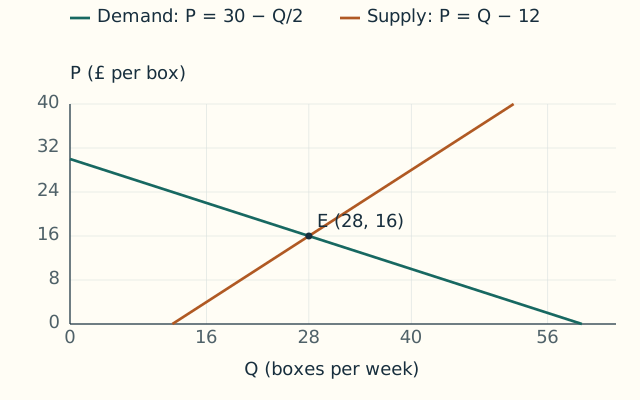
Set the planned quantities equal: 60 − 2P = 12 + P. Subtract 12 and add 2P to get 48 = 3P. Divide by three: P = £16. Substitute into either schedule: Q = 28 boxes per week. Check both: 60 − 32 = 28 and 12 + 16 = 28.

Equilibrium is where both plans agree: 28 boxes per week at £16 per box.
Walkthrough and explanation

Step one writes the equilibrium condition: quantity demanded equals quantity supplied. Step two collects the constant terms on one side and price terms on the other. Starting with 60 minus 2P equals 12 plus P, subtracting 12 gives 48 minus 2P equals P. Adding 2P gives 48 equals 3P. Step three divides both sides by three to obtain 16 pounds per box. Step four substitutes this price into both original equations. Both give 28 boxes per week, so the calculation is internally consistent. Equality is a model condition, not a guarantee that any actual price instantly adjusts to it.

Next slide

Slide 7 / 14

Worked example: diagnose a shortage

At a price of £12, Qd = 60 − 24 = 36 boxes, while Qs = 12 + 12 = 24 boxes. Excess demand is twelve boxes per week. This is a shortage at that price: planned purchases exceed planned sales. It is different from scarcity, which exists even when the market clears.

Walkthrough and explanation

First evaluate both schedules at the same price and over the same period. Second subtract supplied quantity from demanded quantity: 36 minus 24 equals 12. That difference measures unmatched purchase plans, not necessarily a recorded queue of exactly twelve boxes. Actual sales may be limited by available supply and by matching or other frictions. Buyers might compete through higher offers, waiting or search effort. Which adjustment occurs depends on the market’s rules. Scarcity remains at the equilibrium too, because producing and buying notebooks still uses resources that have alternative uses even when no excess demand appears in this model.

Next slide

Slide 8 / 14

Worked example: diagnose a surplus

At £20, quantity demanded is twenty boxes and quantity supplied is thirty-two. Excess supply is twelve boxes per week. Sellers’ plans exceed buyers’ plans at that price. A surplus does not mean the goods have no possible use; it means the specified price and conditions do not reconcile those purchase and sale plans.

Walkthrough and explanation

Calculate demand as 60 minus twice 20, which gives 20. Calculate supply as 12 plus 20, which gives 32. Subtract demand from supply: 32 minus 20 equals 12. Some sellers may cut prices, reduce output, store goods or seek other buyers. Our static model does not specify the speed or exact process of adjustment. Nor does a planned surplus prove that twelve physical boxes have already been produced and wasted. Supply is a planned quantity at a price; the timing of production and whether unsold inventories exist require additional information.

Next slide

Slide 9 / 14

Worked example: a demand shift

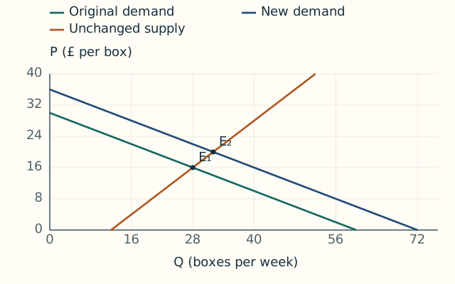
Suppose demand becomes Qd = 72 − 2P while supply remains Qs = 12 + P. At each price, buyers now want twelve additional boxes. Equilibrium satisfies 72 − 2P = 12 + P, giving P = £20 and Q = 32. Demand shifted; the resulting price change causes movement along unchanged supply.

An outward demand shift moves equilibrium from (28, 16) to (32, 20).
Walkthrough and explanation

Step one identifies what changed: the demand intercept rises from 60 to 72, while its price coefficient and the entire supply schedule remain unchanged. Step two equates the new demand with the old supply. Rearranging gives 60 equals 3P, so price is 20. Step three substitutes: 12 plus 20 gives 32 boxes. Compared with the original equilibrium, price rises by four pounds and quantity by four boxes. Quantity demanded also changes, but calling this only a movement along demand misses the initial change in conditions. The equilibrium comparison uses two different demand curves.

Next slide

Slide 10 / 14

Worked example: a supply contraction

Return to original demand, Qd = 60 − 2P. Now supply becomes Qs = 6 + P, six fewer boxes at each price. Equating schedules gives 60 − 2P = 6 + P, so P = £18 and Q = 24. A contraction of supply raises price and lowers equilibrium quantity in this model.

Walkthrough and explanation

Begin from the original baseline rather than silently carrying forward the previous demand shift. The new equality rearranges to 54 equals 3P, which gives a price of 18. At that price, demand is 60 minus 36, or 24 boxes. Supply is 6 plus 18, also 24. Relative to the original price of 16 and quantity of 28, price increases by two pounds and quantity falls by four boxes. The higher price partly offsets the supply contraction through movements along the schedules. It does not undo the underlying loss of supply at each given price.

Next slide

Slide 11 / 14

Several changes can occur together

If demand rises while supply falls, both changes tend to raise price in this model. Their quantity effects oppose one another, so quantity’s direction cannot be inferred without relative magnitudes. With Qd = 72 − 2P and Qs = 6 + P, equilibrium is £22 and twenty-eight boxes, the original quantity at a higher price.

Walkthrough and explanation

Combine the two shifted schedules and solve rather than adding verbal predictions mechanically. Seventy-two minus 2P equals six plus P becomes 66 equals 3P, so price is 22. Supply then gives six plus 22, or 28 boxes. Demand gives the same result. In this particular numerical case, the quantity effects exactly offset. Other shift sizes could raise or lower quantity. A qualitative diagram often identifies some directions but leaves others ambiguous. Saying that an effect is ambiguous without additional information is a valid analytical conclusion, not a failure to understand the model.

Next slide

Slide 12 / 14

Observations do not identify the cause automatically

A higher observed price and quantity are consistent with a demand increase under an unchanged upward-sloping supply curve. They do not prove that demand was the only thing that changed. Quality, income, costs, seasonality and market boundaries may also differ. A causal explanation needs a justified account of what moved and what stayed fixed.

Walkthrough and explanation

Two observed transactions cannot reveal an entire demand curve if demand or supply shifted between them. For example, a festival could increase both the number of buyers and sellers’ staffing costs. Observed price and quantity would reflect both mechanisms. To investigate causality, look for evidence about the changes in relevant conditions, a credible comparison group, or a research design that separates influences. Even then, report uncertainty. The phrase “holding other things constant” is a condition of a model comparison; it is not something we can assume simply because a spreadsheet records only price and quantity.

Next slide

Slide 13 / 14

Equilibrium is not a moral verdict

Market clearing means planned demand equals planned supply under specified conditions. It does not establish justice, adequate information, equal opportunity or absence of harm to outsiders. Efficiency claims need additional assumptions about competition, rights, information and external effects. Whether an outcome should be accepted also depends on values beyond this equality.

Walkthrough and explanation

A price can clear a market even when some people cannot afford the product, when ownership is disputed, or when production imposes pollution costs on neighbours. Those issues are not disproved by the intersection of two curves. Under particular competitive assumptions, economists can make stronger claims about gains from trade and allocation, but the assumptions must be stated. A liberty-oriented perspective may prioritise voluntary exchange and secure rights; another perspective may weigh distribution differently. Clear analysis separates the mechanism that determines an outcome from the ethical reasons for supporting, changing or rejecting the institutions around it.

Next slide

Slide 14 / 14

Use the model carefully

Define the good, period and units. Write the demand and supply schedules and their valid ranges. Solve for equality and check both sides. For any proposed price, distinguish shortage from surplus. When conditions change, identify the shifted schedule before calculating a new equilibrium. Finally, state assumptions, uncertainty and questions the model leaves unanswered.

Walkthrough and explanation

A diagram and an equation can tell the same story if they use consistent axes and definitions. Conventionally, price appears on the vertical axis and quantity on the horizontal axis, even though our equations express quantity as a function of price. You can practise without a graph by checking quantities at several prices. The exercises use new schedules and require explicit numerical answers. Reflection fields are ungraded: they are a place to explain which conditions must remain fixed or why observed correlations are insufficient. Avoid converting a correct algebraic solution into an unsupported claim about a real market.

Go to the exercises

Questions students ask

This guided dialogue explains common sticking points. It is written teaching material, not a live chat service.

If price rises and purchases fall, has demand decreased?

Not necessarily. If the other conditions of demand are unchanged, this is a decrease in quantity demanded along the same schedule. A decrease in demand means a change in the schedule itself.

Is scarcity the same as a shortage?

No. Scarcity concerns competing uses of limited resources. A shortage is excess demand at a specified price and can disappear as conditions change, while scarcity remains.

Must real markets always be at equilibrium?

No. Search frictions, contracts, adjustment delays and other features can prevent or slow market clearing. A static equilibrium is a useful conditional benchmark, not a complete description of every transaction.

Apply the lesson

Your exercises

Use the worked examples to learn the method, then submit these different problems. Numerical and choice answers are checked on the server. Written reasoning is saved for your own review and receives no automatic mark.

Your learning account

You can study every lesson and prepare your answers without an account. Signing in enables private submissions when the service is available.

1. Find a new market equilibrium

Illustrative weekly market: Qd = 80 − 3P and Qs = 8 + P. P is pounds per box; quantities are boxes per week. Solve for the equilibrium price and quantity. Use only the non-negative economically relevant range.

Find a new market equilibrium answers

Answers stay in this tab until you submit. This form does not store drafts on your device.

2. Diagnose two quoted prices

Illustrative weekly market: Qd = 90 − 2P and Qs = 10 + 2P. At £15 and separately at £25, identify whether there is a shortage or surplus and calculate its positive magnitude. Treat these as plans at each specified price.

Diagnose two quoted prices answers

Answers stay in this tab until you submit. This form does not store drafts on your device.

3. New buyers enter

Illustrative weekly market: demand changes from Qd = 100 − 2P to Qd = 115 − 2P. Supply remains Qs = 10 + P. Calculate the new equilibrium and identify the initial change.

New buyers enter answers

Answers stay in this tab until you submit. This form does not store drafts on your device.

4. A loss of available output

Illustrative weekly market: Qd = 96 − 3P and initial Qs = 16 + P. A cost change reduces quantity supplied by twelve units at every price, leaving the slope unchanged. Calculate the new equilibrium. Then explain, in the ungraded field, why observing a higher price alone would not prove that this cost change caused it.

A loss of available output answers

Saved ungraded. Explain your reasoning in your own words.

Answers stay in this tab until you submit. This form does not store drafts on your device.

Your recent submissions

Only submissions for this lesson appear here. Your account export includes your saved attempts.