Course materials are available. Sign-in, submission checking and saved learning records are not open yet. You can read, watch, download and prepare answers in this tab; answers are not saved.

ECON-101 · Lesson 5 of 8

Production, costs and feasible profit

Connect production increments to costs, contribution, operating choices and capacity without confusing cash receipts with economic gains. All scenarios are illustrative.

Allow approximately 65 minutes, including exercises. Work at your own pace.

What you will learn

  • Calculate total, marginal and average product.
  • Distinguish fixed, variable, avoidable and sunk costs for a stated decision.
  • Reconcile cash surplus, economic contribution and economic surplus.
  • Calculate break-even and check workforce or sales choices against capacity.

Watch and work along

Narrated walkthrough

This 11-minute video works through every slide using a clearly identified generic synthetic narrator. It is not a recording of Craig Wright. Captions are always visible below the slide. Pause whenever you need time to calculate. On a small screen, use full-screen playback or the readable text below.

Jump to a slide in the video

The complete lesson

Slide-by-slide walkthrough

Read each slide, follow its explanation, and pause at the examples. The text below supplies the complete written walkthrough, so you can read and recalculate at your own pace.

Slide 1 / 14

Production transforms scarce resources

Production combines labour, equipment, materials, knowledge and time into goods or services. Output is a physical or service quantity; revenue is money received for selling it. More output is not automatically more profit or greater social value. Every business, price and production relationship in this lesson is an illustrative teaching assumption.

Walkthrough and explanation

A workshop can produce more chairs yet earn less if additional chairs sell cheaply or require costly overtime. It can also earn money while imposing a cost on people outside the transaction. Keep three questions separate: what can be produced, what the producer gains, and what happens to everyone affected. We begin with the technical relationship between inputs and output, then add prices and opportunity costs. This sequence makes it easier to see which conclusions arise from technology and which depend on markets, alternatives and values.
Next slide

Slide 2 / 14

A production function holds some things fixed

A production function describes attainable output from specified inputs under a given technology. In a short-run example, equipment is fixed while labour can vary. “Short run” means at least one relevant input cannot adjust; it is not a universal number of months. Long-run comparisons allow all relevant inputs to change.

Walkthrough and explanation

Imagine a workshop with one cutting machine and different numbers of workers. Adding a worker can change how effectively the machine is used, but adding a second machine is outside this particular short-run choice. A different business may adjust equipment much faster or slower. The distinction is about available adjustment, not a fixed calendar rule. The production relationship also assumes comparable worker hours, skill and material quality. If those change across observations, a higher output cannot automatically be attributed to worker numbers alone.

Next slide

Slide 3 / 14

Worked example: marginal product

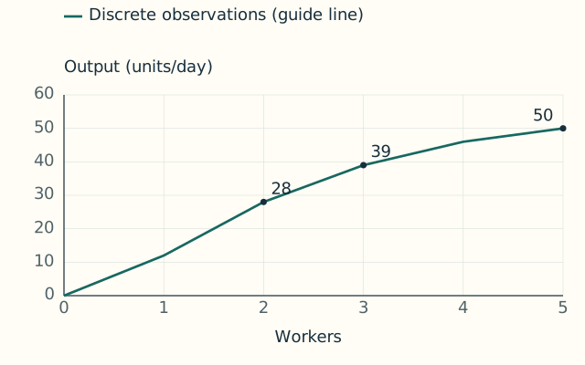
With zero through five workers, illustrative daily output is 0, 12, 28, 39, 46 and 50 units. Each additional worker therefore adds 12, 16, 11, 7 and 4 units. These increments are marginal products. Marginal product starts falling after the second worker, although total output continues rising throughout the table.

Total output rises even after marginal product starts falling after worker two. Worker counts are discrete observations; connecting segments are visual guides.
Walkthrough and explanation

Subtract each output from the next one. The first worker adds 12 minus zero. The second adds 28 minus 12, or 16. The third adds 39 minus 28, or 11. The fourth adds seven and the fifth adds four. Early specialisation can explain an initial rise in marginal product; crowding around fixed equipment can explain a later decline. These are possible mechanisms, not facts established merely by the table. Diminishing marginal product means smaller additions to output, not necessarily falling total output or a judgement about any worker’s individual worth.

Next slide

Slide 4 / 14

Average and marginal product differ

Average product is total output divided by the number of workers. In the same example, three workers produce thirty-nine units, so average product is thirteen units per worker. The third worker’s marginal product is eleven. Adding an increment below the previous average pulls the average down; an increment above it raises the average.

Walkthrough and explanation

At two workers, output of 28 gives an average of fourteen. The third worker adds eleven units, below fourteen, so the new average falls to thirteen. This is a general property of averages. A new observation below an existing average lowers that average when weights are comparable. Average product and marginal product answer different questions: output per worker across the whole team versus output added by a change in team size. Neither alone determines the profit-maximising workforce, because we also need output prices, labour costs and any other costs caused by expansion.

Next slide

Slide 5 / 14

Classify costs along separate dimensions

A fixed cost does not vary with output over the relevant range; a variable cost does. An avoidable cost changes if the activity is stopped; a sunk cost cannot now be recovered. These distinctions are independent. A future monthly subscription can be fixed with respect to sales yet avoidable if the business does not operate.

Walkthrough and explanation

Do not use fixed and sunk as synonyms. Suppose a workshop can cancel next month’s room hire at no charge. The hire is fixed over the month’s feasible production range, but avoiding it is relevant to whether the workshop opens. A non-refundable design payment made last year is sunk for today’s decision. A machine already owned may still have a resale or rental alternative, creating an opportunity cost even if no new cash payment is needed. Classify costs for the specific decision and period rather than attaching permanent labels without context.

Next slide

Slide 6 / 14

Cash surplus is not economic surplus

Cash surplus subtracts the stated cash outlays from receipts. Economic surplus also deducts the value of resources used instead of their best feasible alternatives. An owner’s unpaid time can therefore matter. Define the measure and comparison before using “profit”. Do not subtract an opportunity cost twice when comparing complete alternative plans.

Walkthrough and explanation

If an owner could earn money elsewhere during the same hours, business receipts alone do not show whether operating improves their position. One method subtracts forgone alternative earnings from the business cash surplus. Another adds remaining alternative earnings to business receipts and compares that full allocation with working elsewhere throughout. Both should agree when they include the same costs and time. An accounting allocation may or may not reflect a relevant sacrifice. Ask whether the decision changes cash spending, resource use or the value of an available alternative.

Next slide

Slide 7 / 14

Worked example: contribution per unit

An illustrative product sells for £18. Each unit needs £7 of materials and delivery plus twelve minutes of the owner’s time. Alternative work pays £15 per hour. Twelve minutes is 0.2 hours, worth £3. Economic contribution per unit is therefore £18 − £7 − £3 = £8 before monthly fixed costs.

Walkthrough and explanation

Begin with consistent time units. Divide twelve minutes by sixty to obtain 0.2 hours. Multiply by the available alternative hourly return of fifteen pounds, giving a three-pound opportunity cost per unit. Subtract both the seven-pound cash cost and this time cost from the selling price. Eight pounds remains to cover the costs that do not vary with unit volume and then provide an economic surplus. This contribution assumes each extra sale leaves other sales unchanged, uses the stated resources and fits within capacity. It is not yet the profit on an entire month.

Next slide

Slide 8 / 14

Worked example: build the monthly result

The same business has £90 of avoidable monthly cash costs and four maintenance hours. At £15 per hour, fixed economic costs total £150. Thirty sales give thirty times £8 minus £150, or £90 economic surplus. Cash surplus is £240, but ten total working hours have an opportunity cost of £150.

Walkthrough and explanation

Check the result by two routes. The contribution route gives 30 times eight, or £240, less fixed economic costs of £90 plus four times £15, yielding £90. The cash route begins with 30 times £18 revenue, or £540. Subtract £210 variable cash costs and £90 monthly cash costs to get £240. Production takes thirty times 0.2 hours, or six hours, and maintenance takes four more. Ten hours valued at £15 cost £150 in forgone earnings. Subtracting that from cash surplus gives the same £90 economic result.

Next slide

Slide 9 / 14

Break-even depends on the decision

With £8 contribution per unit and £150 avoidable fixed economic costs, monthly economic break-even is 150/8 = 18.75 units. Nineteen whole sales exceed that threshold under the assumptions. The minimum price for one additional sale after fixed commitments are unavoidable is a different question from the volume needed to justify operating.

Walkthrough and explanation

Write economic surplus as eight times quantity minus 150. Set it equal to zero, add 150 to both sides and divide by eight. The result is 18.75, which is a planning boundary rather than a possible whole-unit sale count. At eighteen units, contribution is £144 and the business is six pounds short. At nineteen, contribution is £152 and the surplus is two pounds. This threshold assumes unchanged prices, costs and product mix. If contribution were zero or negative, increasing volume alone would not cover positive fixed costs within this linear model.

Next slide

Slide 10 / 14

Past expenditure does not force future production

Suppose the owner previously paid £300 for a design that cannot be refunded or sold. That payment is sunk for next month’s operating decision. It may matter when evaluating the original investment, but it does not change next month’s alternatives. Future avoidable costs and current resale opportunities still belong in the comparison.

Walkthrough and explanation

A project can have been disappointing overall and still be worth continuing from today, or have done well historically and now be worth stopping. The relevant question is what each available decision changes. Sunk-cost reasoning does not require forgetting the past: past results can inform forecasts and reveal mistakes. It requires separating information from an unrecoverable payment. Also check whether something described as sunk really is unrecoverable. If the design could be licensed to someone else only when unused by this business, that alternative would create a current opportunity cost.

Next slide

Slide 11 / 14

Capacity makes algebra conditional

The owner has twenty hours available. Four maintenance hours leave sixteen production hours. At 0.2 hours per unit, capacity is eighty units. A formula predicting profitable sales beyond eighty is outside the stated feasible set. Expansion would need another assumption about hours, equipment, productivity or outsourcing, with its associated costs.

Walkthrough and explanation

Subtract fixed time before dividing by time per unit: twenty minus four is sixteen, and sixteen divided by 0.2 is eighty. At full capacity, an extra order cannot simply consume another otherwise unused twelve minutes. It may displace an existing order, require overtime or require someone else’s help. Its opportunity cost must reflect that actual alternative. A constant-contribution formula is useful only while its resource and pricing assumptions hold. Always check a proposed break-even or switching threshold against capacity before presenting it as a feasible business plan.

Next slide

Slide 12 / 14

Worked example: choose a workforce

Return to outputs 0, 12, 28, 39, 46 and 50. Output sells for £12 per unit; each worker costs £100 per day. An already committed £60 daily cost is unavoidable now. Net results for zero through five workers are −£60, −£16, £76, £108, £92 and £40. Three workers is best.

Walkthrough and explanation

Multiply each output by twelve, then subtract one hundred pounds per worker and the committed sixty pounds. For three workers, revenue is 39 times twelve, or £468; costs are £300 plus £60, leaving £108. The fourth adds seven units worth £84 but costs £100, reducing the result by £16. The fifth also reduces it. The first three additions increase the result, even though the one-worker total remains negative after the committed cost. This example shows why marginal contributions and complete-plan comparisons work together. The conclusion assumes all listed staffing options are feasible.

Next slide

Slide 13 / 14

Profit guides choices under specific conditions

Economic profit can signal that resources earn more here than in their stated alternatives. It can encourage entry and imitation where feasible. Losses can encourage adjustment or exit. These mechanisms depend on information, competition and institutions; profit is not a complete measure of social contribution or proof that every cost has been borne privately.

Walkthrough and explanation

A business may discover a useful way to serve customers, or it may benefit from restricted entry, misleading information or costs imposed on others. The same accounting label cannot distinguish those cases by itself. A liberty-oriented approach values experimentation and voluntary cooperation, while a careful analysis asks how rights, liability and competition shape the available opportunities. Long-run entry can reduce some excess returns, but barriers, innovation and uncertainty can sustain differences. Avoid turning a useful tendency into a promise that all markets instantly reach identical returns or perfectly reward social value.

Next slide

Slide 14 / 14

Audit the production decision

State output units, technology, relevant period and feasible inputs. Calculate marginal and average product separately. Classify costs by what the decision changes, including opportunity costs. Reconcile contribution and complete-plan calculations. Test break-even against capacity, and distinguish a marginal order from opening, continuing or expanding an entire operation.

Walkthrough and explanation

A good business calculation should be reproducible by someone who knows only the assumptions and arithmetic. Label pounds per unit, hours per month and total pounds distinctly. Show intermediate values before rounding and explain whether an average represents expected product mix or actual sales. Then test the assumptions most likely to reverse the choice, such as demand, service time or the availability of alternative work. The numerical exercises check specified calculations. Their ungraded reflection fields ask you to identify what the arithmetic leaves unresolved rather than pretending that an automatic marker can fully assess business judgement.

Go to the exercises

Questions students ask

This guided dialogue explains common sticking points. It is written teaching material, not a live chat service.

Does a fixed cost belong in a decision about one extra order?

Only if that order changes it. A cost fixed over the relevant range can still matter when deciding whether to operate for the whole period.

Is unpaid owner labour free?

It has no wage payment, but may sacrifice a valuable alternative. Identify the next-best feasible use rather than automatically valuing it at zero or an unavailable wage.

Does diminishing marginal product mean a worker produces nothing?

No. The additional output can remain positive while becoming smaller. The table describes the whole production arrangement with specified fixed inputs, not an intrinsic measure of a person’s worth.

Apply the lesson

Your exercises

Use the worked examples to learn the method, then submit these different problems. Numerical and choice answers are checked on the server. Written reasoning is saved for your own review and receives no automatic mark.

Your learning account

You can study every lesson and prepare your answers without an account. Signing in enables private submissions when the service is available.

1. Read a new production table

Illustrative daily output at zero through four workers is 0, 15, 33, 45 and 52 units. Calculate the third worker’s marginal product and average product with three workers.

Read a new production table answers

Answers stay in this tab until you submit. This form does not store drafts on your device.

2. Build an economic surplus

Illustrative product: price £24, variable cash cost £9, twelve minutes per unit, alternative earnings £20 per hour. Monthly fixed cash costs are £75 and maintenance takes three hours. At twenty sales, calculate contribution per unit and monthly economic surplus. Also calculate the smallest whole number of sales with a non-negative economic surplus, assuming capacity permits it.

Build an economic surplus answers

Answers stay in this tab until you submit. This form does not store drafts on your device.

3. Respect the time budget

Illustrative business: eighteen hours are available each month, routine maintenance uses three hours, and each order needs fifteen minutes. Calculate normal maximum order capacity. Then calculate switching-month capacity if an additional two hours are required for setup. No extra labour is available.

Respect the time budget answers

Saved ungraded. Explain your reasoning in your own words.

Answers stay in this tab until you submit. This form does not store drafts on your device.

4. Compare feasible staffing plans

Illustrative output with zero through five workers is 0, 10, 24, 33, 39 and 42 units. Each unit sells for £14. A worker costs £80 for the day. An additional £50 is already committed and unavoidable for every staffing choice. Calculate the best workforce and its net result after all stated costs.

Compare feasible staffing plans answers

Saved ungraded. Explain your reasoning in your own words.

Answers stay in this tab until you submit. This form does not store drafts on your device.

Your recent submissions

Only submissions for this lesson appear here. Your account export includes your saved attempts.