Course materials are available. Sign-in, submission checking and saved learning records are not open yet. You can read, watch, download and prepare answers in this tab; answers are not saved.

ECON-101 · Lesson 4 of 8

Elasticity, revenue and who bears a tax

Measure proportional responses, connect demand elasticity to revenue, solve a tax-wedge example and separate causal responses from observed correlations. All examples are illustrative.

Allow approximately 70 minutes, including exercises. Work at your own pace.

What you will learn

  • Calculate signed and absolute midpoint price elasticity with correct bases.
  • Distinguish elasticity from slope and interpret the revenue relationship.
  • Solve a basic per-unit tax model using separate buyer and seller prices.
  • Evaluate the assumptions behind elasticity estimates and causal claims.

Watch and work along

Narrated walkthrough

This 12-minute video works through every slide using a clearly identified generic synthetic narrator. It is not a recording of Craig Wright. Captions are always visible below the slide. Pause whenever you need time to calculate. On a small screen, use full-screen playback or the readable text below.

Jump to a slide in the video

The complete lesson

Slide-by-slide walkthrough

Read each slide, follow its explanation, and pause at the examples. The text below supplies the complete written walkthrough, so you can read and recalculate at your own pace.

Slide 1 / 14

Percentage changes make responses comparable

A change of ten units means different things in a market selling twenty units and one selling ten thousand. Percentages express a change relative to a base. Elasticity compares percentage changes in two variables. All data in this lesson are illustrative. Distinguish a percentage change in a rate from a percentage-point change.

Walkthrough and explanation

If a quantity rises from 50 to 55, the change is five units and the starting-base percentage increase is five divided by 50, or ten per cent. If an interest rate rises from four per cent to five per cent, it rises by one percentage point but by 25 per cent relative to its initial value. These are different measures. Elasticity uses proportional changes, allowing comparisons across units such as boxes, kilograms or litres. Always identify the relevant base and sign before calculating. A calculator cannot correct an ambiguous definition of the percentage you intend to measure.
Next slide

Slide 2 / 14

Demand elasticity is a conditional response

Price elasticity of demand is the percentage change in quantity demanded divided by the percentage change in own price, along an unchanged demand relationship. Ordinary downward-sloping demand gives a negative signed elasticity. We usually classify its absolute magnitude: above one is elastic, below one is inelastic, and exactly one is unit elastic.

Walkthrough and explanation

An elasticity of minus two means that, locally, a one per cent price increase is associated with about a two per cent reduction in quantity demanded, other relevant conditions unchanged. The absolute magnitude is two. Be explicit about whether you report the signed value or its magnitude. Elastic does not mean that quantity is high; it means quantity responds proportionally more than price. An inelastic response is not necessarily zero. Perfectly inelastic demand has zero quantity response in the specified model and range, a much stronger condition than merely having a magnitude below one.

Next slide

Slide 3 / 14

Worked example: use the midpoint method

Price rises from £10 to £12 and quantity falls from 100 to 80 units on one demand curve. Average price is £11; average quantity is 90. Midpoint changes are 2/11 = 18.18% and −20/90 = −22.22%. Signed elasticity is −1.222 approximately; its magnitude exceeds one, so this interval is elastic.

Walkthrough and explanation

Step one calculates the changes: price increases by two pounds and quantity decreases by twenty units. Step two calculates the average of each pair of endpoints: eleven pounds and ninety units. Step three divides each change by its own average, giving approximately 0.1818 and negative 0.2222. Step four divides the quantity proportion by the price proportion. The result is negative eleven-ninths, or approximately negative 1.222. Using midpoint bases gives the same magnitude when the direction of comparison is reversed. Do not divide a percentage quantity change by a raw pound change; that would not be an elasticity.

Next slide

Slide 4 / 14

Revenue connects price and quantity

Total revenue equals price multiplied by quantity sold. In the preceding example, revenue changes from £1,000 to £960. The price rise is outweighed by the quantity response. Along unchanged demand, an elastic interval makes price and revenue move in opposite directions; an inelastic interval makes them move in the same direction.

Walkthrough and explanation

Calculate revenue independently to check the interpretation: ten pounds times one hundred is one thousand pounds; twelve times eighty is nine hundred and sixty. Revenue falls by forty pounds. For positive endpoints, the midpoint elasticity classification is consistent with this finite-change revenue test. If its magnitude is exactly one, the two endpoint revenues are equal. The relationship assumes the observed quantity change is a movement along unchanged demand and that all units sell at the stated price. Revenue is not profit. Costs, returns, discounts and capacity constraints may change whether a pricing decision benefits the seller.

Next slide

Slide 5 / 14

Worked example: an inelastic price cut

Price falls from £20 to £18 while quantity rises from 50 to 54. Average price is £19 and average quantity is 52. The midpoint elasticity is (4/52) divided by (−2/19), approximately −0.731. Revenue falls from £1,000 to £972: the percentage quantity gain is too small to offset the price reduction.

Walkthrough and explanation

First take the signed changes: quantity rises by four and price falls by two. Divide by the midpoint bases to get about positive 7.692 per cent and negative 10.526 per cent. Dividing those proportions gives negative nineteen-twenty-sixths, approximately negative 0.731. Its magnitude is below one, so demand over this interval is inelastic. Next calculate revenues: 20 times 50 equals 1,000, while 18 times 54 equals 972. The price cut reduces revenue by £28. More customers or more units sold therefore does not necessarily imply more sales revenue, still less more profit.

Next slide

Slide 6 / 14

A straight line can have changing elasticity

Slope compares changes in units; elasticity compares proportional changes. For Q = 200 − 10P, the slope is always minus ten units per pound. Point elasticity is −10P/Q. At P = £5 and Q = 150 its magnitude is one-third; at P = £15 and Q = 50 it is three.

Walkthrough and explanation

The same ten-unit response is a larger percentage of a small starting quantity than of a large one. Likewise, a one-pound change is a smaller percentage of a high price than of a low price. That is why a constant slope need not imply constant elasticity. The point formula multiplies the quantity response per pound by price divided by quantity. At five pounds, it gives negative ten times five divided by 150. At fifteen pounds, it gives negative ten times fifteen divided by fifty. Point elasticity describes a small local change; midpoint elasticity summarises an interval between two distinct observations.

Next slide

Slide 7 / 14

Substitution and time influence responsiveness

Demand often responds more when close substitutes are available, when spending represents a larger budget share, or when buyers have time to adjust. These are tendencies to investigate, not universal numerical laws. A narrowly defined product can face more substitutes than a broad category. Essential uses do not make every quantity completely unresponsive.

Walkthrough and explanation

A particular café may have many nearby substitutes, while coffee as a broad category has fewer close alternatives for some customers. Buyers may respond to a lasting fuel-price change by changing routes, vehicles or housing, even if tomorrow’s commute barely changes. The relevant time horizon therefore matters. Different groups can also have different responses. An average market elasticity can conceal people who have few short-run alternatives. To use an estimate responsibly, check its product definition, population, period, price range and research design. An elasticity borrowed from a different setting may be a poor guide.

Next slide

Slide 8 / 14

Supply has an elasticity too

Price elasticity of supply compares the percentage change in quantity supplied with the percentage change in the price received by sellers, other supply conditions unchanged. It is often positive. Capacity, inventories, input availability and time to expand matter. Demand responsiveness and supply responsiveness jointly determine how a market adjusts to a disturbance.

Walkthrough and explanation

A bakery with unused ovens may increase output quickly, while a fully booked venue cannot create more seats for tonight merely because offers rise. Over a longer period, investment or entry can make supply more responsive. These examples concern conditional responses, not shifts caused by new technology or input-price changes. As with demand, distinguish a local elasticity from an estimate over a large interval. A vertical supply curve means fixed quantity in the model’s relevant range, whereas a horizontal curve represents an extremely responsive supply at the given price. Neither shape is appropriate for every market.

Next slide

Slide 9 / 14

Other elasticities answer other questions

Income elasticity relates quantity demanded to income. A positive value describes a normal good; a negative value describes an inferior good over the relevant range. Cross-price elasticity relates demand for one good to another good’s price. Positive responses can indicate substitutes; negative responses can indicate complements, with relevant conditions held fixed.

Walkthrough and explanation

Do not interpret all elasticities as own-price demand elasticity. If bus fares rise and train demand increases, the cross-price response can indicate substitution between travel options. If printer prices rise and demand for ink falls, the goods may be complements. These labels depend on the context and level of aggregation; they are not timeless characteristics of every individual’s preferences. Income elasticity also varies across groups and income ranges. The word inferior has no moral meaning here. As always, an observed correlation is not automatically a causal response when incomes, prices and other conditions move together.

Next slide

Slide 10 / 14

A tax introduces a price wedge

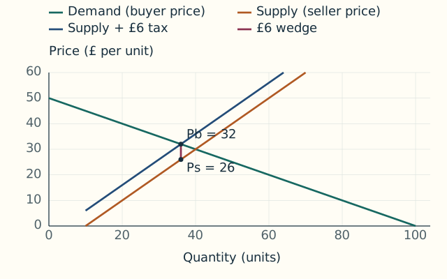
For a per-unit tax, distinguish the price buyers pay, Pb, from the net price sellers receive, Ps. With a £6 tax, Pb = Ps + 6. Our illustrative schedules are Qd = 100 − 2Pb and Qs = 10 + Ps. Without the tax, one common price is £30 and quantity is forty.

Walkthrough and explanation

Before introducing the tax, set buyer and seller prices equal to P. Equilibrium is 100 minus 2P equals 10 plus P, giving 90 equals 3P and P equals 30. Supply then gives 40 units. With the tax, using a single price in both original schedules would erase the distinction we need to analyse. Buyers respond to the amount they pay, while sellers respond to what they retain per unit after the tax. We assume a competitive market, compliance, unchanged underlying schedules and no separate administrative costs or other policy effects.

Next slide

Slide 11 / 14

Worked example: calculate tax incidence

Substitute Pb = Ps + 6 into demand: 100 − 2(Ps + 6) = 10 + Ps. This simplifies to 78 = 3Ps, so Ps = £26 and Pb = £32. Quantity is thirty-six. Compared with the untaxed price, buyers pay £2 more and sellers receive £4 less per unit.

At 36 units buyers pay £32 and sellers receive £26; the vertical wedge is £6.
Walkthrough and explanation

Expand the left side carefully: 100 minus 2Ps minus 12 equals 10 plus Ps. Subtract ten and collect price terms to obtain 78 equals 3Ps. Dividing by three gives 26, then adding the six-pound tax gives the buyer price of 32. Check quantities: demand is 100 minus 64, or 36; supply is 10 plus 26, also 36. Tax revenue is six times 36, or £216. The buyer and seller burdens per traded unit sum to the tax: two plus four equals six. This is a particular model calculation, not a general two-to-one incidence rule.

Next slide

Slide 12 / 14

Legal payment and economic burden can differ

Who sends a tax payment to the authority need not determine who bears its economic cost. In the simple competitive model, the less responsive side generally bears more of a small tax’s price burden. At the untaxed equilibrium here, supply elasticity is 0.75 and demand’s magnitude is 1.5, consistent with sellers bearing more.

Walkthrough and explanation

Use the local elasticity formulas at the original price of 30 and quantity of 40. Supply’s slope is one, so its elasticity is one times 30 divided by 40, or 0.75. Demand’s slope is negative two, giving magnitude two times 30 divided by 40, or 1.5. Sellers are less responsive in this example. This intuition concerns relative ability to adjust quantities. Market power, evasion, price regulation, cross-border options and longer-run changes can alter the result. A positive incidence calculation also does not decide whether a tax is justified; that judgement needs stated goals, rights and other consequences.

Next slide

Slide 13 / 14

A correlation is not a demand experiment

A hot weekend can increase both cold-drink prices and sales. That does not establish an upward-sloping demand curve; demand may have shifted. To estimate a causal price response, isolate a price change from other influences. Randomised prices or credible quasi-experimental variation can help, but each design needs assumptions, appropriate permissions and careful interpretation.

Walkthrough and explanation

Imagine comparing a quiet rainy Tuesday with a crowded sunny Saturday. Weather, visitors, opening hours and stock could differ alongside price. Dividing the observed percentage quantity change by the observed price change gives a descriptive ratio, but not necessarily demand elasticity. A controlled comparison might hold other conditions more nearly constant, while a research design may use a source of price variation unrelated to demand changes. Neither method is automatically flawless. Check selection, spillovers, measurement, compliance and the range of prices studied. Report uncertainty rather than presenting a single estimate as a universal behavioural constant.

Next slide

Slide 14 / 14

Calculate, interpret, then qualify

Name the response being measured. Use consistent percentage bases and report whether elasticity is signed or absolute. Check revenue directly when relevant, and separate revenue from profit. For incidence, distinguish buyer and seller prices. Finally, ask whether other conditions were genuinely controlled and whether the estimate applies to the decision at hand.

Walkthrough and explanation

A reliable answer has three layers. First comes arithmetic: changes, averages, ratios and units. Second comes interpretation: what the magnitude means for the specified demand or supply relationship. Third comes identification and scope: why the data support a causal statement and where the estimate might fail to transfer. The exercises deliberately include a case where arithmetic is possible but a causal demand interpretation is not established. Written reflections remain ungraded. Use them to explain assumptions and evidence, because checking a number cannot substitute for understanding the model or the way the observations were generated.

Go to the exercises

Questions students ask

This guided dialogue explains common sticking points. It is written teaching material, not a live chat service.

Should I report a negative elasticity or a positive one?

State the convention. Signed own-price demand elasticity is normally negative for downward-sloping demand. Elastic, inelastic and unit-elastic classifications commonly use its absolute magnitude.

Can a price cut increase sales and reduce revenue?

Yes. With inelastic demand over the interval, the proportional quantity increase is too small to offset the proportional price reduction. Calculate price times quantity at both endpoints to check.

Can the party legally paying a tax pass all of it on?

That is not automatic. In the simple competitive model, the division depends on demand and supply responsiveness. Other market institutions and adjustment mechanisms can also matter.

Apply the lesson

Your exercises

Use the worked examples to learn the method, then submit these different problems. Numerical and choice answers are checked on the server. Written reasoning is saved for your own review and receives no automatic mark.

Your learning account

You can study every lesson and prepare your answers without an account. Signing in enables private submissions when the service is available.

1. Calculate an interval response

Illustrative unchanged demand curve: price rises from £8 to £10 and quantity falls from 150 to 120 units. Calculate the absolute midpoint elasticity and total revenue at each endpoint. Round elasticity to two decimal places if needed.

Calculate an interval response answers

Answers stay in this tab until you submit. This form does not store drafts on your device.

2. Evaluate another price cut

Illustrative unchanged demand curve: price falls from £30 to £27 and quantity rises from 200 to 210. Calculate absolute midpoint elasticity to two decimal places, the signed change in revenue (after minus before), and the elasticity classification.

Evaluate another price cut answers

Answers stay in this tab until you submit. This form does not store drafts on your device.

3. Solve a new tax wedge

Illustrative competitive market: Qd = 120 − 3Pb and Qs = 12 + Ps. A per-unit tax of £8 creates Pb = Ps + 8. Calculate the buyer price, seller net price and quantity after the tax. All schedules remain unchanged apart from this wedge.

Solve a new tax wedge answers

Saved ungraded. Explain your reasoning in your own words.

Answers stay in this tab until you submit. This form does not store drafts on your device.

4. Separate a ratio from a causal estimate

Illustrative café observations: on a quiet weekday, price is £4 and sales are 80 drinks; during a busy festival, price is £5 and sales are 100. Calculate the signed midpoint percentage-change ratio (quantity change divided by price change). Then decide what the observations alone establish about causal own-price demand elasticity.

Separate a ratio from a causal estimate answers

Saved ungraded. Explain your reasoning in your own words.

Answers stay in this tab until you submit. This form does not store drafts on your device.

Your recent submissions

Only submissions for this lesson appear here. Your account export includes your saved attempts.