Course materials are available. Sign-in, submission checking and saved learning records are not open yet. You can read, watch, download and prepare answers in this tab; answers are not saved.

MATH-100 · Lesson 4 of 4

Coordinates, Straight Lines and Feasible Regions

Connect algebra to a graph, calculate slopes and intercepts, identify combinations that satisfy constraints and separate a graphical pattern from a causal explanation.

Allow approximately 85 minutes, including exercises. Work at your own pace.

What you will learn

  • Read and plot ordered pairs using labelled axes and consistent scales.
  • Calculate and interpret the slope and intercepts of a straight line.
  • Represent linear inequalities as feasible regions with included or excluded boundaries.
  • Distinguish movements along a line, shifts of a relationship and unsupported causal interpretations.

Watch and work along

Narrated walkthrough

This 12-minute video works through every slide using a clearly identified generic synthetic narrator. It is not a recording of Craig Wright. Captions are always visible below the slide. Pause whenever you need time to calculate. On a small screen, use full-screen playback or the readable text below.

Jump to a slide in the video

The complete lesson

Slide-by-slide walkthrough

Read each slide, follow its explanation, and pause at the examples. The text below supplies the complete written walkthrough, so you can read and recalculate at your own pace.

Slide 1 / 14

A graph connects two quantities

A coordinate graph has a horizontal axis and a vertical axis. Label each axis with its variable and unit. Their crossing is the origin, usually (0, 0). A point represents a pair of values. In this lesson, draw simple graphs on paper as you read; the instructions specify the coordinates and boundaries you need.

Walkthrough and explanation

A graph is another language for the relationships we have been calculating. One position records two values at once, allowing us to see patterns that are harder to notice in a list. Start every drawing by naming the quantities on the axes. “Quantity, in kilograms” and “cost, in pounds” are more useful labels than x and y alone. We conventionally put x horizontally and y vertically, but economic graphs may use other variable names or particular axis conventions. Read the labels rather than assuming. Every numerical graph in this lesson is an invented teaching model, not evidence about an actual market.
Next slide

Slide 2 / 14

Ordered pairs and consistent scales

An ordered pair (x, y) gives the horizontal value first and the vertical value second. To plot (3, 7), move to x = 3, then to y = 7. Choose equally spaced tick marks on each axis. The two axes may use different scales, but each individual linear scale must stay consistent.

Walkthrough and explanation

“Ordered” matters because reversing the entries usually places a point somewhere else. Three across and seven up is different from seven across and three up. If negative values are allowed, move left for negative x and down for negative y. Choose scales that fit the relevant values comfortably on the page. For example, each horizontal tick could represent one unit while each vertical tick represents five pounds. That is perfectly valid when labelled clearly. However, switching halfway along one axis from increments of five to increments of ten would distort an ordinary linear graph unless a special break or different scale were explicitly explained.

Next slide

Slide 3 / 14

Build points from a formula

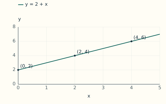
For y = 2 + x, choose values of x and calculate the matching y values. If x = 0, y = 2; if x = 2, y = 4; if x = 4, y = 6. Plot (0, 2), (2, 4) and (4, 6). A linear relationship places these points on one straight line.

Plot the calculated pairs; the line y = 2 + x passes through all three.
Walkthrough and explanation

A small value list is a bridge between algebra and a graph. Substitute each horizontal value into the formula and preserve the matching pair. Three points are useful because the third can reveal an arithmetic or plotting error, even though two distinct points determine a straight line. If the variable can take every intermediate value, connect the points with a straight line over the permitted range. If only whole-number quantities are possible, individual admissible points have the literal meaning; the connecting line is a useful model guide. Do not extend a line beyond the domain without checking whether the formula still applies there.

Next slide

Slide 4 / 14

Slope means vertical change per horizontal change

The slope of a non-vertical straight line is m = (y₂ − y₁)/(x₂ − x₁). It measures the change in y for one unit of x. Between (1, 5) and (4, 11), m = (11 − 5)/(4 − 1) = 6/3 = 2. Subtract coordinates in the same point order.

Walkthrough and explanation

The subscripts simply label the first and second points. They do not mean multiplication or powers. We calculate the vertical difference and divide it by the horizontal difference. In this example, moving three units right raises the vertical value by six, so each horizontal unit corresponds to two vertical units. You may subtract the first point from the second or reverse both subtractions; either gives the same slope. Reversing only one subtraction gives the wrong sign. Keep units: if y is cost in pounds and x is quantity in units, the slope is pounds per unit, not a unit-free number.

Next slide

Slide 5 / 14

Intercepts locate the crossings with axes

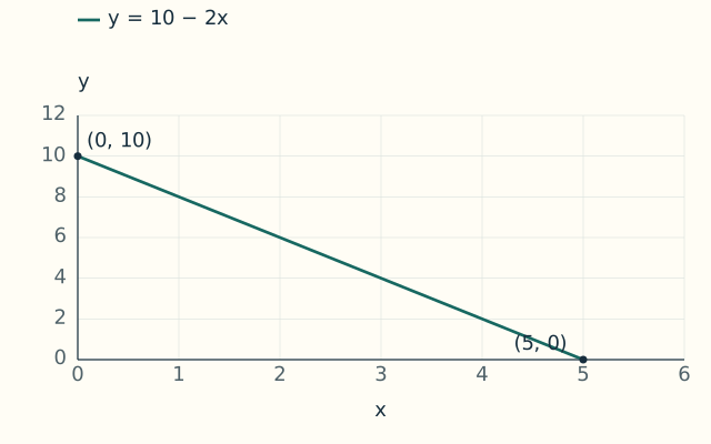
An intercept is where a graph crosses an axis. In y = b + mx, b is the y-intercept because x = 0 gives y = b. To find the x-intercept, set y = 0 and solve. For y = 10 − 2x: y-intercept = 10; 0 = 10 − 2x gives x-intercept = 5.

The intercepts of y = 10 − 2x are (0, 10) and (5, 0).
Walkthrough and explanation

The two intercepts require different substitutions. On the vertical axis the horizontal coordinate is zero, so set x to zero. On the horizontal axis the vertical coordinate is zero, so set y to zero. In our example the crossings are the points zero comma ten and five comma zero. The slope is minus two, meaning a one-unit horizontal increase is associated with a two-unit vertical decrease. An algebraic intercept may lie outside the meaningful domain. A cost line with a positive fixed charge and positive slope, for instance, might have a negative horizontal intercept that does not describe a feasible production quantity.

Next slide

Slide 6 / 14

Positive, negative, zero and undefined slopes

A positive slope rises from left to right; a negative slope falls. A horizontal line has slope zero because y does not change. A vertical line has undefined slope because its horizontal change is zero, which would require division by zero. Visual steepness also depends on axis scales, so compare calculated slopes with their units.

Walkthrough and explanation

Do not confuse a negative slope with a negative value. A falling line can remain entirely above the horizontal axis. Similarly, a rising line can include negative vertical values. Slope describes how values change, not where the line sits. A horizontal line has no vertical change, so its slope is zero divided by a non-zero horizontal change. A vertical line has the opposite issue: the horizontal denominator is zero, so its slope is undefined rather than zero. Finally, stretching the drawing vertically can make the same relationship look steeper. Numerical slopes and stated units protect against misleading visual comparisons.

Next slide

Slide 7 / 14

Movement along a line versus a changed line

Changing x within an unchanged equation moves the point along the existing line. Changing an equation's parameter changes the relationship itself. In y = b + mx, increasing b shifts the line upwards without changing its slope. Changing m changes the slope. Keep these two kinds of change separate when interpreting economic diagrams.

Walkthrough and explanation

Consider a cost relationship with a fixed charge and a constant per-unit charge. Ordering more units under the same charges moves us along the existing cost line. Increasing the fixed charge changes the cost associated with every quantity, so the entire line shifts upwards. Increasing the per-unit charge instead changes how quickly cost rises with quantity; the line becomes steeper when the axis scales stay fixed. This distinction is important because an observed point moving upwards does not by itself tell us which mechanism occurred. We need to know whether quantity changed, the underlying terms changed, or both changed at once.

Next slide

Slide 8 / 14

Worked example: plot an illustrative cost line

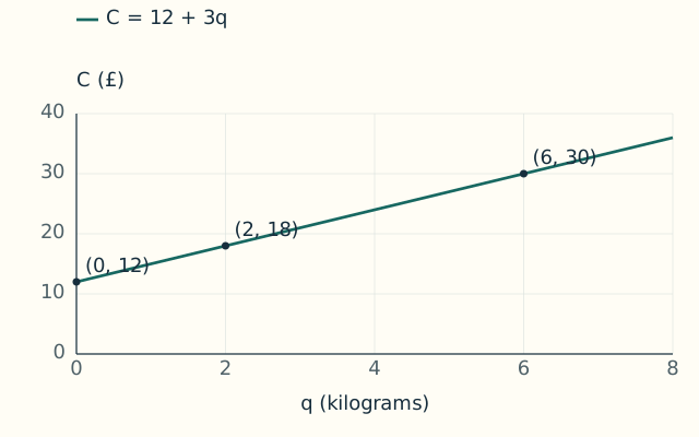
A fictional delivery service charges C = 12 + 3q, where C is pounds and q is kilograms delivered. For q = 0: C = 12 + 3 × 0 = 12. For q = 2: C = 12 + 6 = 18. For q = 6: C = 12 + 18 = 30. Plot (0, 12), (2, 18), (6, 30).

A £12 fixed charge plus £3 per kilogram produces a straight cost line.
Walkthrough and explanation

Draw quantity in kilograms horizontally and total cost in pounds vertically. A horizontal range from zero to six and a vertical range from zero to thirty will include all three points. Mark equal steps on each axis, then locate the calculated pairs. The zero-quantity point represents the fixed charge built into this illustrative formula; whether such a charge would really be payable with no delivery depends on the actual service terms. Here it is part of the stated model. Because kilograms are divisible, the relationship includes intermediate quantities. Join the points with a straight line over the non-negative quantity range being considered.

Next slide

Slide 9 / 14

Worked example: interpret the slope and intercept

Using (2, 18) and (6, 30), slope = (30 − 18)/(6 − 2) = 12/4 = £3 per kilogram. The vertical intercept is £12. Algebra gives the horizontal intercept: 0 = 12 + 3q; −12 = 3q; q = −4. That negative mass lies outside the delivery model's non-negative domain.

Walkthrough and explanation

The slope calculation recovers the coefficient of q, which is a useful check that our plotted values are consistent with the formula. Four additional kilograms raise cost by twelve pounds, so each kilogram adds three pounds. The intercept of twelve pounds is the model's fixed charge, not the price per kilogram. Solving for a horizontal intercept produces minus four kilograms. This is a valid feature of the unrestricted mathematical line, but it is not a possible delivery mass. Draw the meaningful non-negative part as the model, and explain rather than physically interpreting any extension into negative quantities.

Next slide

Slide 10 / 14

Worked example: draw a budget boundary

An illustrative £48 budget buys beans at £6 per kilogram and rice at £4 per kilogram. Let x be kilograms of beans and y kilograms of rice. Affordable combinations satisfy 6x + 4y ≤ 48, with x ≥ 0 and y ≥ 0. The full-spending boundary is 6x + 4y = 48.

Walkthrough and explanation

We are now graphing two goods rather than a quantity and its cost. Put beans on the horizontal axis and rice on the vertical axis. Each combination has a total cost: six pounds times bean kilograms plus four pounds times rice kilograms. The budget allows spending less than or exactly forty-eight pounds, which explains the less-than-or-equal sign. To draw the boundary, temporarily replace that sign with equality. Set y to zero: six x equals forty-eight. Divide both sides by six: x = 48 ÷ 6 = 8. Set x to zero: four y equals forty-eight. Divide both sides by four: y = 48 ÷ 4 = 12. Join the intercepts eight comma zero and zero comma twelve.

Next slide

Slide 11 / 14

Worked example: choose the affordable side

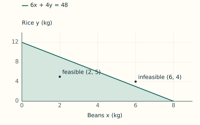
Boundary intercepts are (8, 0) and (0, 12). Test (2, 5): cost = 6 × 2 + 4 × 5 = 12 + 20 = £32 ≤ £48, so it is feasible. Test (6, 4): cost = 36 + 16 = £52 > £48, so it is infeasible. Shade the first-quadrant region on or below the boundary.

The shaded region contains all non-negative bundles costing no more than £48.
Walkthrough and explanation

A feasible combination satisfies every stated restriction. The first test point spends thirty-two pounds and leaves sixteen pounds unused, so it lies inside the affordable region. The second spends fifty-two pounds and exceeds the budget by four pounds. The origin is also affordable because buying neither good costs zero in this model. Use a solid boundary because equality is included: combinations spending exactly forty-eight pounds are allowed. Rearranging the boundary gives four y equals forty-eight minus six x, then y equals twelve minus one point five x. Its slope means an extra kilogram of beans requires giving up one point five kilograms of rice when spending remains at the budget limit.

Next slide

Slide 12 / 14

Several constraints mean an intersection

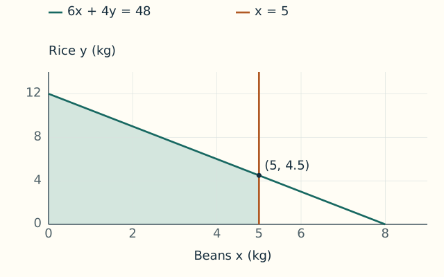
A feasible region must satisfy all constraints together. Add x ≤ 5 to the previous budget model. At x = 5, the budget boundary gives 6 × 5 + 4y = 48, so 4y = 18 and y = 4.5. The remaining region has corners (0, 0), (5, 0), (5, 4.5), (0, 12).

Intersect the budget region with x ≤ 5; the new corner is (5, 4.5).
Walkthrough and explanation

The additional restriction might represent a five-kilogram availability limit in this invented scenario. Draw the vertical line x equals five and retain only points to its left, including the line itself. Then keep only points that also satisfy the budget and non-negativity conditions. The word “and” is important: satisfying one constraint is insufficient. The four listed corners outline the intersection. Fractional coordinates are acceptable here because kilograms are divisible. With indivisible items, only permitted whole-number points within the region would describe actual choices. A feasible region shows what is allowed; it does not identify a best choice until an objective or preference is specified.

Next slide

Slide 13 / 14

Read a graph without claiming too much

Check axis labels, units, scale, time period and the range shown. Association means quantities vary together; causation means a change in one produces a change in another. A graph alone usually cannot establish causation. A truncated vertical axis can magnify apparent changes, and extending a line beyond observed or modelled values can be unreliable.

Walkthrough and explanation

A graph can be arithmetically accurate while encouraging a mistaken impression. Starting the vertical axis near the smallest plotted value can make a modest difference look dramatic, so inspect the tick labels rather than judging height alone. Distinguish a theoretical relationship based on stated assumptions from a scatter of observed values. Observed quantities may move together because a third factor affects both, because influence runs in the opposite direction, or because of selection and chance. Interpolation uses the relationship within its supported range; extrapolation extends beyond that range. Neither a straight line nor a neat pattern guarantees that such an extension will remain valid.

Next slide

Slide 14 / 14

A graph-reading and drawing checklist

Name the variables and units; choose consistent scales; calculate and plot reliable points; identify slope and relevant intercepts; state the domain. For inequalities, draw the boundary and test a point to select the correct side. Combine all restrictions. Finish with a sentence explaining what the picture supports and what it cannot establish.

Walkthrough and explanation

Connect this routine to the earlier lessons. Units tell you what each axis means. Algebra supplies the points, intercepts and constraints. Ratios underlie slope, while percentage changes offer a different way to compare movements when the base is known. For an inequality with a strict symbol, use a dashed boundary to show that equality is excluded; for an inclusive symbol, use a solid boundary. A test point should not lie on the boundary, because it must distinguish the two sides. In the exercises, calculate from the stated relationships rather than judging a sketch by eye, and keep any causal conclusion within the evidence actually supplied.

Go to the exercises

Questions students ask

This guided dialogue explains common sticking points. It is written teaching material, not a live chat service.

Why is a coordinate written in a particular order?

The first coordinate identifies the horizontal position and the second the vertical position. Reversing them usually changes the point. Axis labels also determine the meaning and units of each coordinate.

Is the steepest-looking line always the one with the largest slope?

Only when the relevant axis scales and units are comparable. Stretching an axis changes apparent steepness. Calculate vertical change divided by horizontal change and retain its units.

Can a feasible point leave some budget unspent?

Yes, when the constraint says spending must be less than or equal to the budget. Equality describes the boundary, while points with lower spending can also be feasible. Other constraints still need to be satisfied.

Does the boundary itself belong to the feasible region?

It belongs when the inequality includes equality, shown by ≤ or ≥. A strict < or > excludes the boundary. A solid line indicates inclusion, while a dashed line indicates exclusion.

Why does a feasible region not tell me the best choice?

Feasibility answers whether a combination is allowed. Choosing the best feasible combination requires an additional objective, such as a stated profit formula or the chooser’s preferences. Different objectives can select different points.

If two quantities rise together, has one caused the other?

The graph shows an association, but that is not enough to establish causation. Other influences, reverse causation or the way observations were selected may explain the pattern. Additional evidence and a justified method are needed.

Apply the lesson

Your exercises

Use the worked examples to learn the method, then submit these different problems. Numerical and choice answers are checked on the server. Written reasoning is saved for your own review and receives no automatic mark.

Your learning account

You can study every lesson and prepare your answers without an account. Signing in enables private submissions when the service is available.

1. Calculate a slope from two points

An invented straight cost line contains the points (1, 8) and (5, 24), where the first coordinate is quantity in units and the second is total cost in pounds. Calculate its slope in pounds per unit.

Calculate a slope from two points answers

Answers stay in this tab until you submit. This form does not store drafts on your device.

2. Find both intercepts

Consider y = 18 − 3x. Give the x-coordinate where the line crosses the horizontal axis, and the y-coordinate where it crosses the vertical axis. Enter the coordinates requested, not coordinate pairs.

Find both intercepts answers

Answers stay in this tab until you submit. This form does not store drafts on your device.

3. Find a boundary combination

An invented £60 budget can buy good x at £3 per unit and good y at £5 per unit. Both goods have non-negative whole-number quantities. If exactly 5 units of x are bought, what is the maximum affordable quantity of y?

Find a boundary combination answers

Answers stay in this tab until you submit. This form does not store drafts on your device.

4. Test three candidate combinations

A fictional feasible region is defined by 4x + 3y ≤ 36, x ≥ 0 and y ≥ 0. Classify each point using all three constraints: A = (3, 6), B = (6, 5), C = (9, 0). Points on an included boundary satisfy that constraint.

Test three candidate combinations answers

Answers stay in this tab until you submit. This form does not store drafts on your device.

5. Choose a supported interpretation

Four fictional cafés report these pairs: (outdoor tables, daily drinks sold) = (2, 40), (4, 50), (6, 70), (8, 80). Nothing is reported about café size, location, weather or how cafés were selected. Which conclusion is supported by these observations alone?

Choose a supported interpretation answers

Answers stay in this tab until you submit. This form does not store drafts on your device.

Your recent submissions

Only submissions for this lesson appear here. Your account export includes your saved attempts.